$\require{cancel} \newcommand{\Ket}[1]{\left|{#1}\right\rangle} \newcommand{\Bra}[1]{\left\langle{#1}\right|} \newcommand{\Braket}[1]{\left\langle{#1}\right\rangle} \newcommand{\Rsr}[1]{\frac{1}{\sqrt{#1}}} \newcommand{\RSR}[1]{1/\sqrt{#1}} \newcommand{\Verti}{\rvert} \newcommand{\HAT}[1]{\hat{\,#1~}} \DeclareMathOperator{\Tr}{Tr}$
Grover's Algorithm
First created in August 2018
To find a marked item in an unstructured list (e.g. unsorted), a classical algorithm would take on average $N/2$ runs (minimum 1 and maximum $N$). On a quantum computer, the complexity can be improved to $\sqrt N$ (proven by Bennett, 1997). For a list of 10,000, it is a difference between 5,000 classical runs and 100 quantum runs.
Such search algorithm was discovered by Lov Grover in 1996.
The basic idea is to device a unitary operation, which will amplify the amplitude of the "winning" state.
The Oracle
Let us encode the unstructured list of $N$ items as a series of $n$ qubits. i.e. $N\le 2^n$. To simplify the illustration, we only consider $N=2^n$. (The case of $N<2^n$ is a subset of the problem set.) For example, if we have $N=8$ items, we encode them in $n=3$ qubits ($8=2^3$).
The "winning" state $\Ket w$ is among the basis states $\Ket x\in\{\Ket0,\Ket1\}^n$. The function $f(x)$ will return 1 when $x=w$ and 0 otherwise.
The oracle, $U_f\Ket x=(-1)^{f(x)}\Ket x,~$ is a unitary operation that will negate the winning state $\left(U_f\Ket w=-\Ket w\right)$ or otherwise will do nothing $\left(U_f\Ket x=\Ket x\right)$.
For example, a simple list of two items encoded with $\Ket0$ and $\Ket1$, and the marked item is $\Ket1$, will have $U_f\Ket{0}=\Ket{0}$ and $U_f\Ket{1}=-\Ket{1}$.
$U_f =\begin{bmatrix} 1&0\\ 0&-1\\ \end{bmatrix} .$
If the list is encoded from $\Ket0$ to $\Ket3$ and the marked item is $\Ket2$, then $U_f\Ket{10}=-\Ket{10}$.
$U_f =\begin{bmatrix} 1&0&0&0\\ 0&1&0&0\\ 0&0&-1&0\\ 0&0&0&1\\ \end{bmatrix} .$
If the list is encoded from $\Ket0$ to $\Ket7$ and the marked item is $\Ket5$ (the sixth item), then $U_f\Ket{101}=-\Ket{101}$.
$U_f =\begin{bmatrix} 1&0&0&0&0&0&0&0\\ 0&1&0&0&0&0&0&0\\ 0&0&1&0&0&0&0&0\\ 0&0&0&1&0&0&0&0\\ 0&0&0&0&1&0&0&0\\ 0&0&0&0&0&-1&0&0\\ 0&0&0&0&0&0&1&0\\ 0&0&0&0&0&0&0&1\\ \end{bmatrix} .$
The two-item list above can be visualised on a Bloch Sphere. $U_f\left(\Rsr2(\Ket0+\Ket1)\right)=\Rsr2(\Ket0-\Ket1)$, effectively mapping $\Ket+$ to $\Ket-$, which means $U_f=Z$.
The above example implies that a superposition is to be used for the oracle to work. Otherwise, if only basis states are used for input, it is a classical algorithm.
(The two-item case here is for illustration only, not to show speed up, as the classical algorithm can do it in a single run anyway.)
Amplitude amplification
A uniform superpostion $\Ket s=\frac{1}{\sqrt N}\sum_{x=0}^{N-1}\Ket x$ is a state with an equal projection on each basis state. If you measure $\Ket s$, you will get a 1-in-$N$ chance of finding the marked item (which is classical speed).
The winning state $\Ket w$ and the uniform superposition $\Ket s$ span a two-dimensional plane in $\mathbb{C}^n$. Let us call it the $w$-$s$ plane.
In the 2-item case above, $\Ket w=\Ket1$ and $\Ket s=\Ket+$ span the $Z$-$X$ plane.
In the 4-item case above, $\Ket w=\Ket2$ and $\Ket s=\sqrt{\frac{1}{4}}\big(\Ket0+\Ket1+\Ket2+\Ket3\big).$ (Let us not simplify $\sqrt4$ to $2$, to show $N=4$ explicit.)
The two states $\Ket s$ and $\Ket w$ are not orthogonal. Let $\Ket{s'}$ be a state on the $w$-$s$ plane that is orthogonal to $\Ket w$. i.e. $\Braket{s'\Verti w}=0$, which is $\Ket s$ with $\Ket w$ removed.
In the 2-item case above, $\Ket{s'}=\Ket0=\sqrt2\Ket s-\Ket w$ and $\Braket{s'\Verti w}=0$.
In the 4-item case above, $\Ket{s'}=\Rsr3(\Ket0+\Ket1+\Ket3)$, which is $\sqrt{\frac{4}{3}}\Ket s-\sqrt{\frac{1}{3}}\Ket w$ and $\Braket{s'\Verti w}=0$.
Generally, $\Ket{s'} =\sqrt{\frac{1}{N-1}}\sum_{x=0,x\ne w}^{N-1}\Ket x =\sqrt{\frac{N}{N-1}}\Ket s-\sqrt{\frac{1}{N-1}}\Ket w .~~$ $\Braket{s'\Verti w}=0,$ so $\Ket{s'}$ is orthogonal to $\Ket w$.
To prove: $\mathrm{RHS} =\sqrt{\frac{N}{N-1}}\left(\Rsr N\sum_{x=0}^{N-1}\Ket x\right)-\sqrt{\frac{1}{N-1}}\Ket w =\sqrt{\frac{1}{N-1}}\left(\sum_{x=0}^{N-1}\Ket x-\Ket w\right) =\mathrm{LHS} .$
That means $\Ket{s'}$ is without $\Ket w$. Therefore, $U_f\Ket{s'}=\Ket{s'}.$
Let us express $\Ket s$ in basis $\{\Ket{s'},\Ket w\}$, so $\Ket s=\sqrt{1-\frac{1}{N}}\Ket{s'}+\sqrt{\frac{1}{N}}\Ket w.~~$
$\boxed{\Ket s=\alpha\Ket{s'}+\beta\Ket w, \text{ where }\alpha=\sqrt{1-\frac{1}{N}}\text{ and }\beta=\sqrt{\frac{1}{N}}}.$ Note: $\alpha^2+\beta^2=1.$
In our 2-item case, $N=2, \Ket s=\Ket+, \Ket{s'}=\Ket0, \Ket w=\Ket1.$ We have $\Ket+=\Rsr2\Ket0+\Rsr2\Ket1,$ which is exactly right.
The Process
The following diagram shows the case of $N=4$:
$\Ket{s}=\sqrt{\frac{1}{4}}\big(\Ket{00}+\Ket{01}+\Ket{10}+\Ket{11}\big).~~ \Ket{w}=\Ket{10}.~~ \Ket{s'}=\sqrt{\frac{1}{3}}\big(\Ket{00}+\Ket{01}+\Ket{11}\big).~~ \Ket{s}=\sqrt{\frac{3}{4}}\Ket{s'}+\sqrt{\frac{1}{4}}\Ket w .$
The four states are coded as 1, 2, 3 and 4. (Again, we are not simplifying $\sqrt4=2$, so as to show $N=4$.)
The red arrow in the left diagram has a projection of $\alpha$ on the horizontal axis $\Ket{s'}$ and of $\beta$ on the vertical axis $\Ket w$.
We set the initial state $\Ket{\psi_0}=\Ket s.~~$ Some relationships useful later on: $~\cos\theta=\alpha=\sqrt{1-\frac{1}{N}}~$ and $~\sin\theta=\beta=\sqrt{\frac{1}{N}}~$.
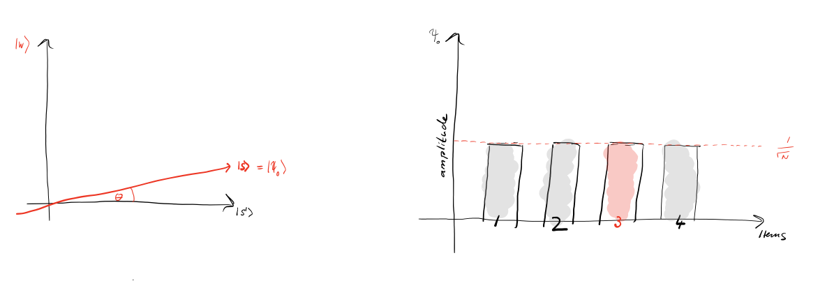
Diagram source: IBM Q Experience.
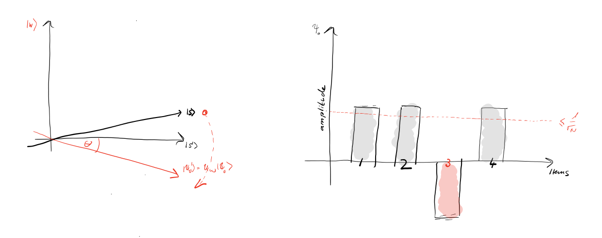
There are two steps in each iteration, the first being to apply $U_f$ to the initial state $\Ket{\psi_0}$ to negate the coefficient of $\Ket w$ and obtain
$\Ket{\psi_0'} =U_f\Ket{\psi_0} =U_f\Ket s =\sqrt{1-\frac{1}{N}}\Ket{s'}-\sqrt{\frac{1}{N}}\Ket w =\alpha\Ket{s'}-\beta\Ket w .$
Geometrically, by negating the coefficient of $\Ket w$, it is effectively to reflect $\Ket{\psi_0}$ on the orthogonal $\Ket{s'}$.
Generally, the reflection operator on $\Ket\phi$ is $U_\phi=2\Ket\phi\Bra\phi-I$. This is by projecting the source vector to $\Ket\phi$, doubling the projection, then subtracting from the source vector to form the target one. (Think of a diamond shape.)
So we have $U_f=2\Ket{s'}\Bra{s'}-I.$
The second step is to reflect $\Ket{\psi_0'}$ on $\Ket s: U_s=2\Ket{s}\Bra{s}-I.$
$\Ket{\psi_1}=U_s\Ket{\psi_0'}=U_sU_f\Ket{\psi_0},~~$ which will be used as the input for the next iteration.
More generally $\Ket{\psi_{t+1}}=U_sU_f\Ket{\psi_t},$ or $\boxed{\Ket{\psi_t}=(U_sU_f)^t\Ket s},~~$ where $t$ is the iteration.
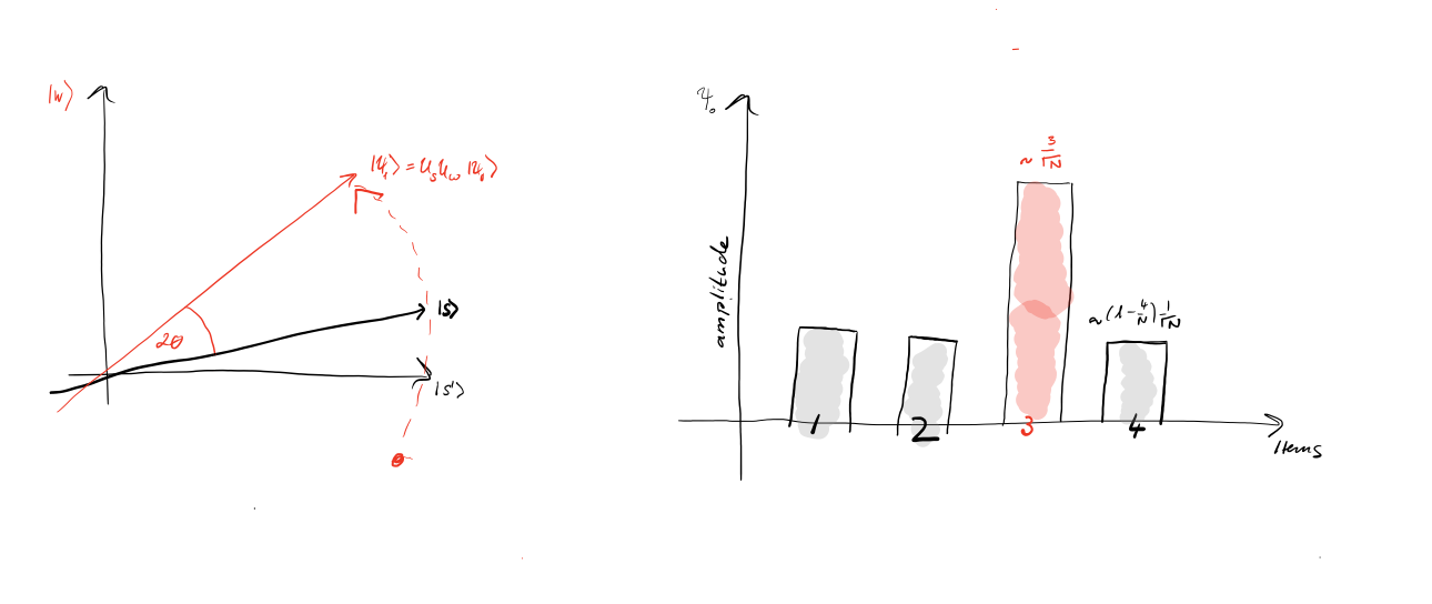
The angle formed by $\Ket{\psi_t}$ and $\Ket{s'}$ would be $\boxed{\theta_t=(2t+1)~\theta}$.
Note: There was a typo at IBM Q Experience that the angle $2\theta$ is between $\Ket{s'}$ and $\Ket{\psi_1}$ as indicated in the IBM Diagram. The correct illustration is to have the $2\theta$ between $\Ket s$ and $\Ket{\psi_1}$, as correctly shown above.
We already have $\boxed{\sin\theta=\sqrt{\frac{1}{N}}}$. When $N$ is large, $\theta\approx\sqrt{\frac{1}{N}}~$, so $\displaystyle\theta_t=(2t+1)\theta\approx\frac{2t+1}{\sqrt N}$ after iterating $t$ times.
To get $\theta_t$ close to $\pi/2,~~$ $\frac{2t+1}{\sqrt N}\approx\pi/2,~~t\approx\frac{\pi}{4}\sqrt N-\frac{1}{2}.~~$ i.e. The complexity is $O\left(\sqrt N\right)$.
An interesting case when $N=4$, where $\sin\theta=\sqrt{\frac{1}{4}}=\frac{1}{2},~~\theta=\frac{\pi}{6}.~~$ When $t=1,~~\theta_1=3\theta=\frac{\pi}{2}~$ exactly, no need for approximation.
The Grover's Algorithm finds the winning state out of four items in a single iteration with absolute certainty! Regardless of complexity, this fact along worth some attention, and will be explored in Grover's Algorithm Analysis.
Implementation
This section is about how to implement $U_sU_f$ with quantum gates.
The strategy is to examine the combined matrix of $U_sU_f$ and see if we can decompose it into Pauli gates.
In general, $\Big[\Ket{\varphi_1}~\Ket{\varphi_2}\Big]A =\big[\Ket{\varphi_1}~\Ket{\varphi_2}\big]\begin{bmatrix}a_{11}&a_{12}\\a_{21}&a_{22}\end{bmatrix} =\Big[a_{11}\Ket{\varphi_1}+a_{21}\Ket{\varphi_2}~~a_{12}\Ket{\varphi_1}+a_{22}\Ket{\varphi_2}\Big] =B\Big[\Ket{\varphi_1}~\Ket{\varphi_2}\Big] .$
Givens:
$\Ket s =\sqrt{1-\frac{1}{N}}\Ket{s'}+\sqrt{\frac{1}{N}}\Ket w =\alpha\Ket{s'}+\beta\Ket w .$
$\Braket{s\Verti s'} =\sqrt{1-\frac{1}{N}} =\alpha.~~ \Braket{s\Verti w} =\sqrt{\frac{1}{N}} =\beta .$
As expected: $\alpha^2+\beta^2=1,~\Braket{s'\Verti w}=\Braket{w\Verti s'}=0.$
The combined operator: $U_sU_f =\big(2\Ket s\Bra s-I\big)~\big(2\Ket{s'}\Bra{s'}-I\big) =4\alpha\Ket s\Bra{s'}-2\Ket s\Bra s-2\Ket{s'}\Bra{s'}+I .$
$U_sU_f\Ket s\\ =\left(4\alpha\Ket s\Bra{s'}-2\Ket s\Bra s-2\Ket{s'}\Bra{s'}+I\right)\Ket s\\ =4\alpha^2\Ket s-2\Ket s-2\alpha\Ket{s'}+\Ket s\\ =(4\alpha^2-1)\Ket s-2\alpha\Ket{s'}\\ =(4\alpha^2-1)\Ket s-2\alpha\left(\frac{1}{\alpha}\Ket s-\frac{\beta}{\alpha}\Ket w\right) =(4\alpha^2-3)\Ket s+2\beta\Ket w=\left(1-\frac{4}{N}\right)\Ket s+\frac{2}{\sqrt N}\Ket w$
$U_sU_f\Ket{s'}\\ =\left(4\alpha\Ket s\Bra{s'}-2\Ket s\Bra s-2\Ket{s'}\Bra{s'}+I\right)\Ket{s'}\\ =4\alpha\Ket s-2\alpha\Ket s-2\Ket{s'}+\Ket{s'}\\ =2\alpha\Ket s-\Ket{s'}$
$=2\alpha\left(\alpha\Ket{s'}+\beta\Ket w\right)-\Ket{s'}\\ =\left(2\alpha^2-1\right)\Ket{s'}+2\alpha\beta\Ket w\\ =\left(1-2\beta^2\right)\Ket{s'}+2\alpha\beta\Ket w .$
$U_sU_f\Ket w\\ =\left(4\alpha\Ket s\Bra{s'}-2\Ket s\Bra s-2\Ket{s'}\Bra{s'}+I\right)\Ket w\\ =-2\beta\Ket s+\Ket w$
$=-2\beta\left(\alpha\Ket{s'}+\beta\Ket w\right)+\Ket w\\ =-2\alpha\beta\Ket{s'}+(1-2\beta^2)\Ket w .$
With reference to orthonormal basis $\{\Ket{s'},\Ket w\}$, $U_sU_f =\begin{bmatrix} 1-2\beta^2&-2\alpha\beta\\ 2\alpha\beta&1-2\beta^2 \end{bmatrix} =(1-2\beta^2)I-2i\alpha\beta Y .$
From Rotation: Matrix Exponentials, when $\displaystyle A^2=I,~~e^{i\varphi A} =I\cos\varphi+iA\sin\varphi,~~$ where $\varphi\in\mathbb{R}.$
$U_sU_f$ is in the same form with $\cos\varphi=(1-2\beta^2),~\sin\varphi=-2\alpha\beta,$ and $A=Y$.
To verify applicability, $Y^2=I$ and $\cos^2\varphi+\sin^2\varphi=(1-2\beta^2)^2+(-2\alpha\beta)^2=1-4\beta^2+4\beta^4+4(1-\beta^2)\beta^2=1.$
To express $\varphi$ in terms of $\alpha$ and $\beta$, let $\beta=\sin\left(\frac{\varphi}{2}\right).~~ 1-2\beta^2=1-2\sin^2\left(\frac{\varphi}{2}\right)=\cos(\varphi).~~ -2\alpha\beta=-2\cos\left(\frac{\varphi}{2}\right)\sin\left(\frac{\varphi}{2}\right)=-\sin(\varphi) .$
We have $U_sU_f =I\cos\varphi-iY\sin\varphi =e^{-i\varphi Y} .$
Rotation in Hilbert space is given by $\varpi_y(\varphi)=e^{-i\varphi Y}.$
Given $\beta=\sin\theta,~~$ we have $\varphi=2\theta,~~$ and therefore $U_sU_f=e^{-i\varphi Y}=e^{-2\theta~iY}~$ means the operation is a rotation of $~2\theta~$ from $\Ket{s'}$ towards $\Ket w$ in each iteration.
Let $\beta_t=\Braket{\psi_t\Verti s'}~$ and $~\theta_t~$ be the angle from $\Ket{s'}$ to $\Ket{\psi_t}$. We have $\sin\theta_t=\beta_t.~~$ (Note: $\theta_t\ne\sin^{-1}\beta_t$ when $\theta_t>\pi/2$.)
To maximise $\beta_t$, we need to choose $t_{final}$ such that $\beta_{t_{final}}$ is closest to $\pi/2$. Given a large $N,~~\beta\approx\theta,~$ and $\displaystyle t_{final}\approx\frac{\pi}{2\theta}\approx\frac{\pi}{2\beta}=\frac{\pi}{2}\sqrt N$.
$\therefore\boxed{\text{Grover's althorithm requires }O\left(\sqrt N\right)\text{ evaluations to reach the optimal solution}.}$